Posts by Collection

courses

00 Course Notes - Reading Order

Course Notes - Reading Order

Derivation of P(s) - Second-Order System

01.2 DC Gain Explained

DC gain is the steady-state output of a system when you apply a constant (DC) input. “DC” comes from electronics-direct current means zero frequency.

01.3 Natural Frequency, Poles, Damping (2nd Order System)

Eigenvalues = Poles

Explanation: Eigenvalues and poles are the same thing!

01.4 Damping Ratio and Resonance

As soon as the damping ratio, $\zeta$ goes below $0.707$, we will start to see resonance. $\zeta = 0.707$ is the smallest value to have a constant $0dB$ effect like the following:

Just one rule to visualize

$20 dB$ is a factor of 10
Hence, $40 dB$ is a factor of 100
$3 dB$ is basically of factor $\sqrt2$ (But $-3 dB$ is a factor of $\frac{\sqrt2}{2}$)
$6 dB$ is a factor of $2$ (But $-6 dB$ is a factor of $0.5$ )
For reference, I am adding the whole table here:

What is an Open-Loop Plant?

02.2 Closed Loop System with Feedback Control

Block Diagram

02.3 Gain Margin and Phase Margin

Let’s say, you have a gain margin of $6+0.1 dB$, what does that mean?

02.4 Controller or Compensator Design

When we are adding a controller/compensator into our system (by system, I mean, the state-space with the observer and with the control gains), what is the transfer function of that controller? By the way, a compensator just means the controller block that sits between the measured plant output and the plant input.

But why would we want a transfer function for controller or compensator?

03.1 Creating a LTI Object in MATLAB - Part 1

There are many ways to create an LTI object in MATLAB. However, the most conventional are two methods.

State-Space to LTI
Transfer Function to LTI In my experience, if you don’t have both the equations- only the ODE, always go for constructing Transfer Function first and then convert it to LTI. Reason is if you don’t know the exact mapping of $y=Cx+Dy$ then you might end up with wrong result.

03.2 Creating a LTI Object in MATLAB - Part 2 (Conversion)

State-Space to Transfer Function

Method 1 (Analytical)

03.3 State-Space Info from LTI Object

If you have an LTI object say, H_sys. And you would like to extract, A, B , C , D matrix, then use the following

03.4 Impulse Response Function Plotting

TODO: HW from Applied Linear System

03.5 sgrid Code for s-plane

``` octave figure; hold on;

03.6 Pole Placement (Const Damping and Const Freq Line) s-plane

03.5 sgrid Code for s-plane

03.7 Drawing Block Diagram in LaTeX

Link: [Courses and Educational Talks

MACS LAB](https://macslab.xyz/teaching/)

04.1 Why Do We Bother with State-Space Realization

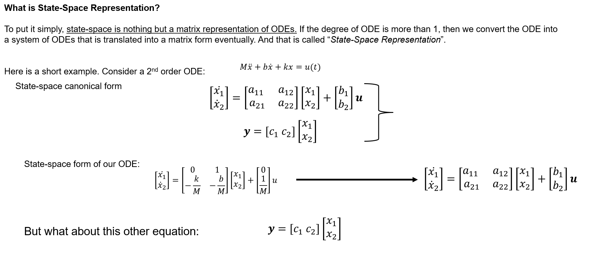
That is a very insightful way to frame it. You’ve hit on the core “engineering” reason why we bother with state-space realizations in the first place. While transfer functions are great for intuition in the frequency domain, state-space is where the heavy lifting happens for complex systems.

04.2 Intuition (Mapping) of State-Space Realization

Pasted image 20260514132135

04.3 Transfer Function Matrix - A Misconception

From 03.1 Creating a LTI Object in MATLAB - Part 1, there might be a misconception that transfer function, $\mathbf{H}$ is a single polynomial. Something like the following:

05.1 Controllability 1

The idea of controllability is best understood through the following example. Again, it all starts with a state-space representation (or, in MATLAB lingo, an LTI object).

05.2 Controllability 2

Once we get the basic intuition from 05.1 Controllability 1, how do we know that if a system is controllable? There are couple of ways actually to do this. They are as follows:

05.3 TODO - Why Observability and Controllability are Dual Problems

05.4 Full State Feedback - Part 1

We start with a state-space system where we have $A,B,C,D$ defined, right? We can refer to the MIMO system mentioned in 04.3 Transfer Function Matrix - A Misconception.

06.1 Luenberger Observer (State Estimation) - Full State Feedback - 2

From 05.4 Full State Feedback - Part 1, we know that control gain, $G$, is applied to all the states, right? But in practice, we typically do not have all the states. So we estimate them. Now, the question is: how do we estimate them?

06.2 Luenberger Observer - 2

MATLAB Implementation of Luenberger Observer and Why this observer problem looks like a 05.4 Full State Feedback - Part 1

06.3 Observer (State Estimator) and Augmented System

We have cleared up the confusion regarding the 06.1 Luenberger Observer (State Estimation) - Full State Feedback - 2. By the way, observer means state estimator!

06.4 Augmented System - 2 with Control Command

Once we complete 06.3 Observer (State Estimator) and Augmented System, we would incorporate the control law into the augmented system.

07.1 Integral Control (LQR) - Part 1

We have come a long way from open-loop plant 01.1 Basics of Open Loop to closed-loop plant 02.2 Closed Loop System with Feedback Control.

07.2 Integral Control (LQR) - Part 2

As we kind of defined why we needed a controller state, now we would like to incorporate that into our augmented system, right? 07.1 Integral Control (LQR) - Part 1