05.1 Controllability 1

The idea of controllability is best understood through the following example. Again, it all starts with a state-space representation (or, in MATLAB lingo, an LTI object).

For example, we have the following state-space system: \(\begin{bmatrix} \dot{x_1}\\ \dot{x_2}\\ \dot{x_3} \end{bmatrix}= \begin{bmatrix} -1 & 0 & 0 \\ 0 & -2 & 1\\ 0 & 2 & -2 \end{bmatrix} \begin{bmatrix} x_1\\ x_2\\ x_3 \end{bmatrix} + \begin{bmatrix} 0&1\\ 1&0\\ 1&0 \end{bmatrix} \begin{bmatrix} u_1\\ u_2 \end{bmatrix}\) \([y] =\begin{bmatrix}1&0&-1 \end{bmatrix} \begin{bmatrix} x_1\\x_2\\x_3 \end{bmatrix}+\begin{bmatrix} 0&0\end{bmatrix}\begin{bmatrix}u_1\\u2 \end{bmatrix}\) Corresponding block diagram of it is the following: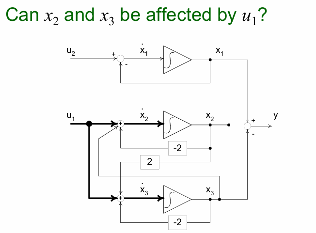

This is the idea of controllability!

Description: That means that you cannot use $u_1$ to affect $x_1$ and $x_2$. That traces back to the core question that can we start from any initial position $\mathbf{x_0}$ to any position $\mathbf{x}$ within a finite time $t_1-t_0$. Now, if you cannot use $u_1$ to drive $x_1$ and $x_2$, you cannot really make this statement of going from one location in space to another location in space!

05.3 Draft - Why Observability and Controllability are Dual Problems